The Degeneracy Distillery

What do DJs and scientists have in common?

With Deaglan Bartlett, Niall Jeffrey & Ben Wandelt

Introduction

Scientists, like DJs, prefer their controls, switches, and dials (physics, ingredients, equations) to be simple, and ideally, independent of one another. In practice, the real world is messy. Data is noisy, people step on cables at the show – when things are going wrong, different switches can often interfere and produce the same output – this is what we call a degeneracy.

Degeneracy: when two or more switches produce similar outcomes in combination.

When models are parameterised by too many switches, they’re often called “sloppy”. James Sethna’s research on Sloppy Models formalises this notion and seeks to reduce the number of control parameters in a problem. But even when you have a small number of parameters, you can still be left with severe degeneracies that make inference (figuring out settings from data) and controlling the system difficult.

Despite the difficulties they present, degeneracies can provide insight about the “physics” or intrinsic properties of a system and its data. The way in which two or more parameters are degenerate is a label for the “physical” or “natural” coordinates that best control the data. In cosmology, a famous example is the \(S_8\) parameter, which captures both how “clumpy” the Universe is, and how much matter it contains.

A Famous Example

\[E = mc^2\]

This equation needs little introduction, but contains the right ingredients to describe what a degeneracy can look like. In this formula, you can change the speed of light, but if you also change the mass of the object by just the right amount, the energy doesn’t change:

This animation shows that the observed energy spectrum (left) changes if mass is varied, but stays fixed if you traverse the “settings” space along curved lines (\(E^*={\rm constant}=mc^2\)), corresponding to changing mass and the speed of light simultaneously.

Hearing Degeneracy

Consider two dials that control the volume (amplitude) of a sound wave. Let’s call the dial settings \(d_1\) and \(d_2\). If we consider a product degeneracy, the output signal might be controlled as

\[\texttt{amp} = d_1 \times d_2 + \textrm{noise}\]

where multiple combinations of \(d_1\) and \(d_2\) produce the same value of \(\texttt{amp}\). Ideally we would “freeze” \(d_2\) and just control the volume with \(d_1\). Now, what if we had three dials ? Or what if there was a nonlinear relationship between the controls, like \(\texttt{amp} = d_1^2 + d_2 + \textrm{noise}\)?

Let’s make the analogy to DJing explicit. Give the interface below a spin. Load your own tracks, or use the built-in synth sound to hear what degenerate controls look and sound like as output sound:

Changing how the switches (parameters) interact with one another impacts how the output sound (data) behaves. In some cases, many different settings produce the exact same output. This effect can be hard to distinguish when the tracks themselves get louder or softer. If you don’t know the mathematical form of the faders’ interference, this can get pretty frustrating if you’re playing a set or trying to distinguish models in the lab!

In cosmology these degeneracies are quite pervasive in fitting theoretical models for the evolution of the Universe to the data that we observe. Different theoretical parameter “twins” can produce the same Cosmic Microwave Background (CMB) data.

Ideally, we would be able to “wire” these controls together into fewer, more independent “master switches”. But how can we do this if all we have are snapshots of the output data (or complicated simulations) and switch settings ?

Can we learn the equation linking the switches together from switch readings and soundwaves alone ?

Distilling Degeneracies from Data

paper link

With the Degeneracy Distillery, the answer is yes. Using just a few snapshots of complicated systems we can distill simple equations that cleanly separate (and sometimes eliminate) interference between switches. We break this down into three steps, using only two main input ingredients: pairs of data and parameters, \(\{ (\textbf{x}, \theta) \}\).

For the illustrations that follow we’ll use a classic, difficult statistics problem to illustrate the distillery. The Rosenbrock function maps a “flat” 2D Gaussian mean, \(\eta=(\nu_1,\nu_2)\), to a degenerate coordinate space \(\theta=(\mu_1,\mu_2)\):

\[\mu_1 = \nu_1, \quad \mu_2 = \nu_2 + \nu_1^2, \quad \Leftrightarrow \quad \nu_1 = \mu_1, \quad \nu_2 = \mu_2 - \mu_1^2\]

Here the data are noise generated from the means \(\theta\) with fixed covariance \(\Sigma\). The data here can be a very long vector: here we draw 50, 2D i.i.d. datapoints per parameter combination, resulting in a 100-dimensional data vector. This toy model is a difficult test problem for probabilistic methods because it yields posteriors \(p(\theta \mid \textbf{x})\) that produce deep “U”-shaped valleys that are difficult to sample or “traverse”. Our goal will be to uncover this “U” shape and learn the mapping \(\eta(\theta)\) from data and \(\theta\) samples alone.

Step 1: Grab data and learn information geometry

Information geometry is how parameter uncertainty changes as the parameters change. We saw this above in our two toy examples: some parts of parameter space lead to bigger changes in data, others lead to smaller or no changes. This is encoded in changes in the likelihood of the data, \(p(\textbf{x}\mid \theta)\).

We can draw a map of where these sensitivities occur. For parameter values that very sensitively control the data, we might imagine the sharp peak of a high mountain, or a “hot” region on a weather heatmap. For regions of parameter space that don’t impact the data much, we might think of a valley or a “cold” spot.

Mathematically, information geometry is described by the Fisher Information Matrix, which forms a metric, or underlying grid. Mathematicians often illustrate metrics locally as an ellipse. For flat regions, the ellipse looks circular (no preferred direction). For a “peak” or a “valley”, we see the ellipse stretched in one preferred direction, indicating a slope or gradient in information space. Explicitly, each element of the Fisher information is given by:

\[F_{ab}({\theta}) = -\int {\rm d}\textbf{x}\ p(\textbf{x} | {\theta})\, \frac{\partial}{\partial {\theta}^a}\frac{\partial}{\partial {\theta}^b} \log p(\textbf{x} | {\theta}),\]

which is usually read as an average over data realisations at a given parameter value.

But how do we obtain this topological map from data and parameters alone? We do this by asking a neural network to compress data into a Fisher matrix and parameter estimate at each point in parameter space, and then minimise the KL divergence for a Gaussian:

\[L_{\rm fish}( \theta, (F_\theta, \hat{\theta})) = \frac{1}{2} (\hat{\theta} - \theta)^T F_\theta (\hat{\theta} - \theta) - \frac{1}{2} \log \det F_\theta\]

One way to think of the Fisher information here is as a “precision”, or inverse-covariance matrix. As the network tries to minimise the error on its predictions, \((\hat{\theta} - \theta)\), it must simultaneously maximise the Fisher information via the second determinant term.

We can see our topological map emerge as a function of training epoch. Each ellipse is a Fisher Matrix centred on a parameter and data vector in a validation set of simulations:

As the networks get better at predicting parameter values from data, the estimated Fisher matrix “bullseyes” shrink at each point. Notice how at the end of training some of the ellipses are different sizes and colours in different parts of parameter space. Brighter, smaller Fisher matrices indicate that the data generated at those coordinates, on average, contain more information about how to distinguish those settings. By contrast, darker, “stretched” Fisher matrices highlight parameter degeneracies. In these regions, the data responds similarly to changes in both parameters. This changing information geometry is precisely what describes difficult-to-resolve physical degeneracies between parameters.

Step 2: Use a neural network to “flatten” the geometry everywhere.

Now that we have a map of the information geometry, we would next like to find a way to “flatten” this space, such that it’s easier to traverse (fields are easier to cross than mountains, even in information-geometry space). Mathematically, this means finding some coordinate system that maps our Fisher matrices to a flat, isometric geometry, defined by the identity matrix in \(n\) parameters, \(\mathbb{I}\). Now that we have an objective, we can work out a loss function for a neural network to optimise. From information geometry, the Fisher matrix transforms from one coordinate system \(\theta\), to another, \(\eta\), via the transformation

\[F_\eta = \frac{\partial \theta}{\partial \eta}^\top F_\theta \frac{\partial \theta}{\partial \eta}.\]

With some rearrangement, we obtain the flattening loss for the Fisher matrix in the new coordinate system,

\[L_{\rm flat} = || J^{-\top} F_{\theta} J^{-1} - \mathbb{I} ||^2_{\mathcal{F}}.\]

This loss forces a neural network, \(\eta_{\rm nn}(\theta)\), to find nonlinear combinations of the original parameters that flattens the mountain range via the coordinate transformation (Jacobian) \(J=\frac{\partial \theta}{\partial \eta_{\rm nn}}\). You can see this coordinate-learning in action below:

After a “burn-in” period, we can see a characteristic “U” shape emerge in \(\eta_1\) (lefthand panel).

Step 3: Use Symbolic Regression to distill degeneracy equations

We now have a neural network that can flatten the learned information geometry. But how can we turn this into “physical” understanding? Symbolic regression is a way to fit a library of symbols and parameters to data in a principled way, much like one fits a line to data by varying a slope and intercept. When the data are very large, like our 100-dimensional rosenbrock data vector, we cannot do this directly from \(\textbf{x}\), since the search space can explode exponentially as the input size increases. However, our neural mapping from parameters to \(\eta\) is now much smaller-dimensional, and captures the important directions of the data via the flattened information geometry. We can now fit symbolic expressions to each neural component \(\eta_j\), and choose simple expressions that distill important, nonlinear relationships among \(\theta\) parameters. For the Rosenbrock case, we uncover:

\[\eta_1 = b_1\mu_1^2 + b_2\mu_2,\;\quad \eta_2 = b_3\mu_2,\]

which is exactly the form we expect by construction. Now that our method is calibrated, we can use it to uncover unkown parameter combinations from data alone! We apply the distillery to difficult parameter combinations in physics, statistics, and epidemiology (like learning infection and recovery rates from COVID-19 data).

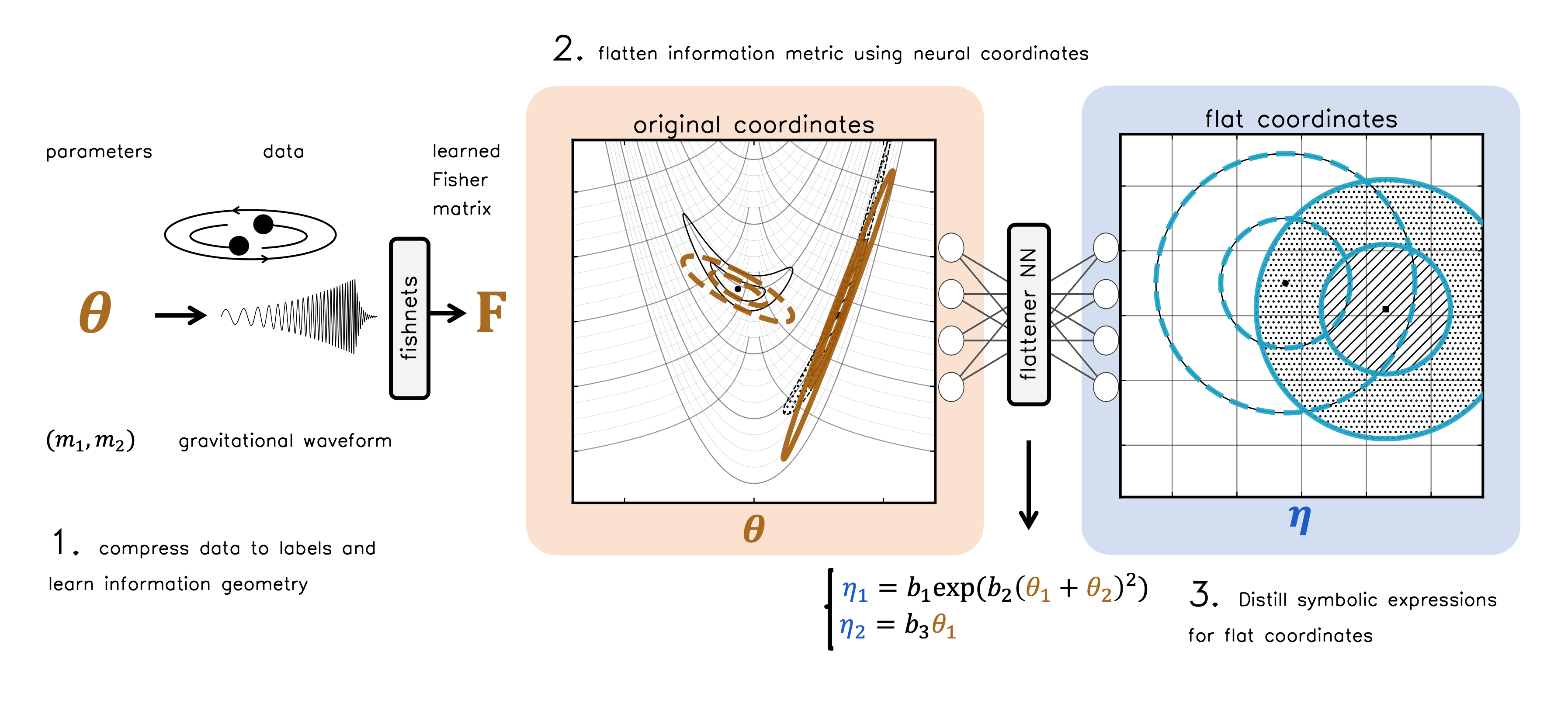
Weighing Black Holes

A toy inspiral gravitational wave binary system and "chirp" waveform data.

My favourite example links back to our DJ decks. Gravitational waves (GWs) are ripples in space-time, similar to how sound waves are ripples in air. When two black holes collide, they form a “chirp” which we can “hear” using massive detectors like LIGO, who record these perturbations using precision lasers kilometers apart. Gravitational wave astronomers can use these waveforms to study the nature of black holes, and most importantly, their masses.

This “chirp” is controlled by the masses of the two black holes, which are degenerate with one another. The “chirp mass” is a nonlinear combination of \(m_1\) and \(m_2\) which dominates simple models of their collision:

\[\mathcal{M}_c = \frac{(m_1 m_2)^{3/5}}{(m_1 + m_2)^{1/5}}\]

Our code finds a version of this formula from chirp waveforms alone when we ask it to disentangle two masses. Beginning with the information geometry, we see that the learned Fisher matrices trace the chirp mass direction:

And the flattener network isolates a nonlinear coordinate that tries to “undo” this degeneracy direction (with a very satisfying “snap” at the end):

Fitting symbolic expressions to the flattener neural coordinates isolates a bijection of the chirp mass and mass ratio \(q=(m_2/m_1)\) coordinates typically used in GW astronomy.

Towards discovery?

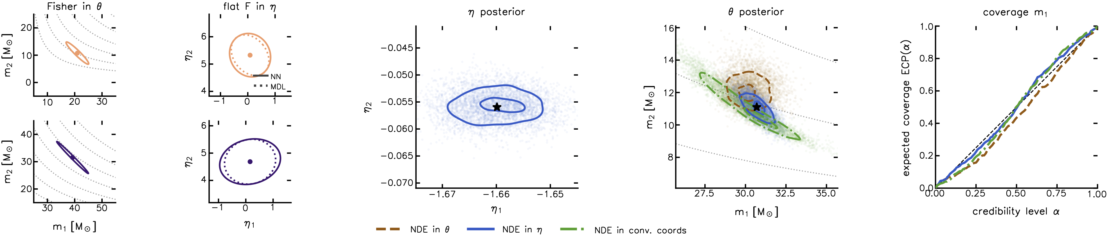
If we upgrade the black hole collision code to be more realistic (more physics and noise in the chirp waveform –like playing a more complicated song in the tapedeck above), this chirp mass no longer dominates – we don’t actually know what degeneracy combination is best to control the signal with \((m_1,m_2)\).

Our code in this case finds simple formulae in terms of total mass and the difference in the two masses:

\[\eta_1 = g(m_1+m_2), \quad \eta_2 = b_0 (m_1-m_2) .\]

When we use this for inference (e.g. trying to “weigh” a gravitational wave binary system with data) we find that these new coordinates are more efficient at describing how the data are controlled by the masses, giving us tighter, better-calibrated results as well as physics intuition about this model and data.

Closing thoughts

The Degeneracy Distillery is a tool to isolate useful and (perhaps) physically-meaningful parameterisations from data. Knowing how data “moves” in terms of physical parameters might help push scientists towards better inference and discovery.

Degeneracies (physically-meaningful coordinates) and their symbolic forms are learnable from data and parameters alone.