Cosmic Graphs: the Language of Large-Scale Structure

how much information is locked inside halo catalogues?

read the paper get the code run in browser

With Tom Charnock, Pablo Lemos, Natalia Porqueres, Alan Heavens, & Ben Wandelt

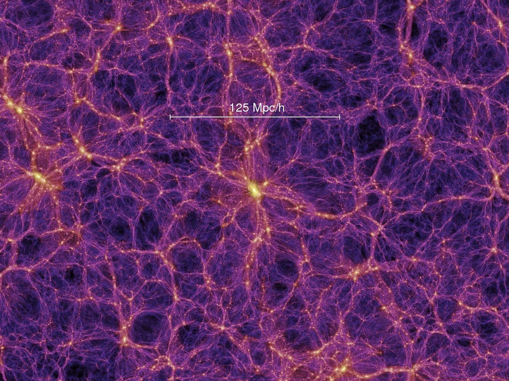
The cosmic web, or Large-Scale Structure (LSS) is the massive spiderweb-like arrangement of galaxy clusters and the dark matter holding them together under gravity. The lumpy, spindly universe we see today evolved from a much smoother, infant universe. How this structure formed and the information embedded within is considered one of the “Holy Grails” of modern cosmology, and might hold the key to resolving existing “tensions” in cosmological theory.

But how do we go about linking this data to theory ? In this project, my team and I will propose to look at LSS assembled as a graph, and use neural networks to optimally extract information about cosmological parameters (theory) from this representation.

Cosmology as an optimization problem

Large-Scale Structure is large. The image below shows a piece of a simulation of the cosmic web ($125\ {\rm Mpc} = 125 \times 10^6$ light years). This massive expanse translates into a lot of data for cosmologists to work with. For context, the European Satellite Euclid will observe billions of galaxies and their properties in an effort to trace the LSS and the dark matter halos forming the cosmic web. Ideally, we’d use the full field-level image of this structure, but this can be challenging when we have billions of pixels.

Cosmology can be thought of as a multigenerational optimization problem, with the objective being:

What statistic (what number(s)) best links LSS data to theory ?

Since the 1960’s, cosmologists have used $n$-point functions to describe structure formation. The image data collected by state-of-the-art surveys are often immediately compressed into (still very large) galaxy and cluster catalogues, whose pairwise (2-point), triplet (3-point), … distances can be compared to quantify how clustered the universe is on different scales.

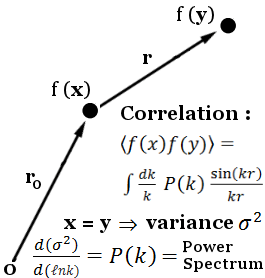
2-point functions are easy to compute even for large data, but don’t capture all the information in highly non-gaussian fields, like the LSS. 3-point functions reclaim a lot of this information, but are much more expensive to compute.

Graphs: a Language for Large-Scale Structure

Graphs provide a natural language with which to describe the cosmic web. Dark matter halos are attributed to nodes (vertices), while filaments are traced by smaller halos and edges. In this representation, clustering under gravitational interactions can be translated into higher edge cardinality (number of edges). Higher order n-point functions can be computed efficiently for clusters, while avoiding the cost of computing extraneous connections across voids. Void catalogues (where edges would correspond to the walls separating the voids) can likewise be assembled into the dual of a halo graph. Graph construction also allows extra information, such as the halo masses, to be added in the form of node and edge labels, unlike correlation functions.

This language is a lot more general – Ben even thought Jim Peebles might have described the cosmic web with graphs if he’d had the resources to do so in 1967.

What is a graph ?

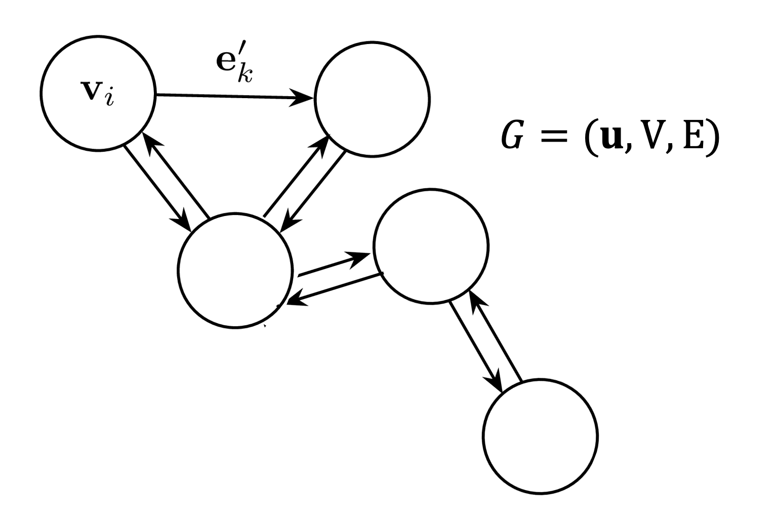
Before we delve into the machinery, let’s define some vocabulary for looking at data on graphs. We can define a graph as a tuple,

$\begin{equation} G = (\textbf{u}, V, E),\label{eq:graphdef} \end{equation}$ where $\textbf{u}$ is a global attribute of the graph, i.e. a label or global parameter value and $E$ and $V$ are the set of edges and nodes, respectively. The edge set

\[E = \{({\bf e}_k, r_k, s_k) \}_{r_k = i, k=1:N^e},\]

indexed by $k=1:N^e$, is comprised of vectors ${\bf e}_k$ of cardinality $N^e$, which may be directed, connected via receiving and sending indices between nodes, $r_k$ and $s_k$. Edges can be equivalently parameterized by an adjacency matrix $A_{ij}$ in which $i$ and $j$ index sender and receiver nodes, respectively. Each node, indexed by $i=1:N^v$, has a set of edges, $E_i$, connected to it via a subset of senders and receivers. The full set of nodes is defined as

\[V= \{\textbf{v}_i \}_{i=1:N^v},\]

where each node $\textbf{v}_i$ is a vector of features. In a physical system of particles, one might represent $V$ as a set of individual particles’ attributes, like mass, position, and velocity, with edges expressing interactions, such as forces, between particles.

Graphs are a really general way to think about arbitrary data representation. For instance, images can be thought of as nodes (pixels) arranged on a 2D lattice (regularly-spaced edges).

Dark Matter Halo Graphs from Catalogues

To create a graph from a catalogue of dark matter halos (or galaxy clusters), we need to define two physical parameters:

a mass cut, $M_{\rm cut}$
a connection radius, $r_{\rm connect}$

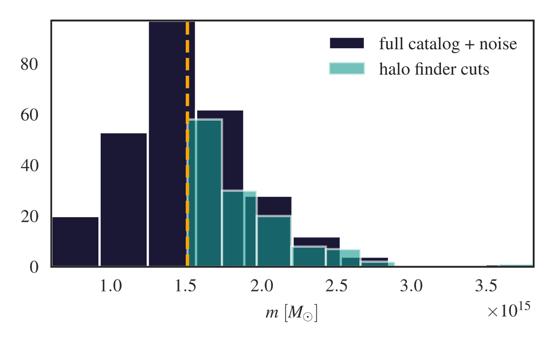
We trunctate a catalogue to halos with a minumum mass $M_{\rm cut}$. We’ll then connect all remaining halos to all other halos within a radius of $r_{\rm connect}$. In Figure 5, the dark points are halos with $M_{\rm cut}=1.5\times10^{15} M_{\rm sun}$, while light points are halos with masses $M_i > M_{\rm cut}=1.1\times10^{15} M_{\rm sun}$.

These two physical parameters change the cardinality of the graph, or the length of the set of edges and nodes, which is now an informative feature about cosmology, as opposed to fixed-length data. The $M_{\rm cut}$ we selected gives us about 100 halos per Quijote simulation – this is a very small dataset, but still contains a wealth of information !

Assembling graphs

One of the goals of this study is to show how graphs can be made more ornate and aid in information extraction about cosmology from detailed dark matter simulations.

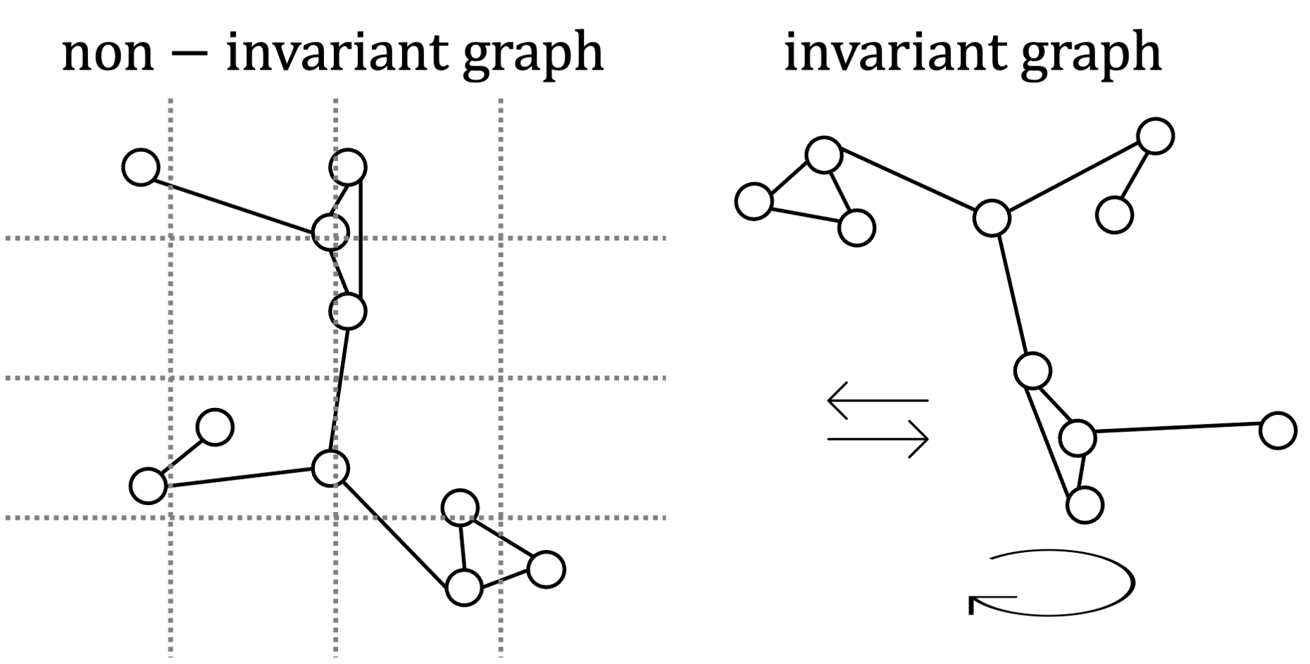
We choose to assemble graphs in two ways: invariant and non-invariant. There has been a lot of research in the GNN community about “inductive biases” – this is just fancy lingo for smart data representation.

The cosmological parameters we want to extract are global properties of the graph, ${\bf u}$, and should be the same if a universe is rotated or translated to another grid, provided the relative structure stays the same.

Encoding these physical symmetries should make pulling out physical information easier, right? We test this hypothesis by using these two representations.

Invariant graphs have all relative positional information (distance and angles) stored in the edges. These graphs are symmetric or invariant under translations and rotations.

\[\begin{align} \textbf{e}_{ij} &= [d_{ij}, \alpha_{ij}, \beta_{ij}]\ &\texttt{# dist, angles between i and j} \\ \textbf{v}_i &= [M_i], &\texttt{# mass} \end{align}\]

Non-invariant graphs are only labelled with relative distance information in the edges, with other positional information stored in the nodes as $(x_i,y_i,z_i)$ coordinates for each halo $i$.

\[\begin{align} \textbf{e}_{ij} &= d_{ij}\ \texttt{# dist between halos i and j} \\ \textbf{v}_i &= [M_i, \textbf{p}_i],\ \texttt{# mass, (x,y,z) position} \end{align}\]

Extracting Information from graphs

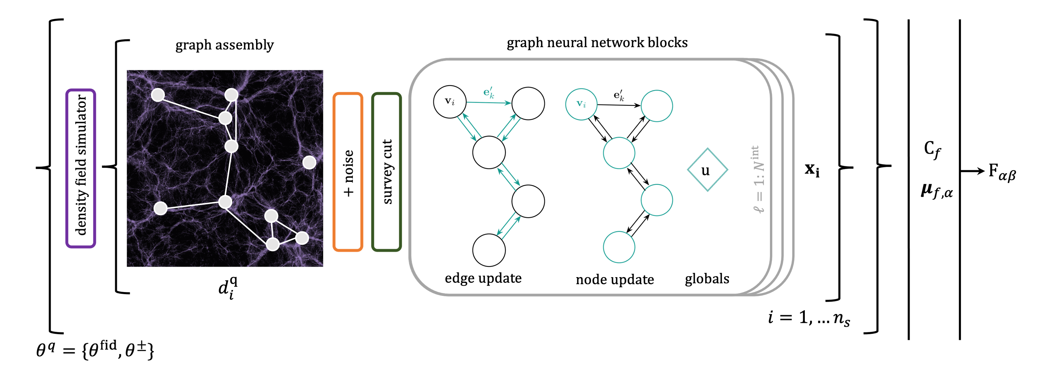
But how do we extract information from a set of edges and nodes whose size changes ? Enter graph Information Maximising Neural Networks (gIMNNs) ! Remember how cosmology can be thought of as an optimization problem to find informative statistics ? IMNNs do precisely that, from simulations !

IMNNs optimizing the Cramer-Rao bound, which describes the average variance (uncertainty) of estimates of parameters $\vartheta$:

\[\langle (\vartheta_\alpha - \langle \vartheta_\alpha \rangle )(\vartheta_\beta - \langle \vartheta_\beta \rangle) \rangle \geq \textbf{F}^{-1}_{\alpha \beta}\]

By maximising the Fisher information of some distribution, $\textbf{F}$, we minimize the uncertainty in the parameters, better constraining the theory.

IMNNs do this automatically by learning $f: \textbf{d} \rightarrow \textbf{x}$, a mapping $f$ from some big data $\textbf{d}$ to a small set of summaries $\textbf{x}$. We use neural networks to learn $f$, since these can be trained via backpropagation on data !

To do this, and without loss of generality (proof coming soon!) we compute a Gaussian likelihood form to compute our Fisher information:

\[\begin{equation} -2 \ln \mathcal{L}(\textbf{x} | \textbf{d}) = (\textbf{x} - \boldsymbol{\mu}_f(\vartheta))^T \textbf{C}_f^{-1}(\textbf{x} - \boldsymbol{\mu}_f(\vartheta)) \end{equation}\]

where $\boldsymbol{\mu}_f$ and $\textbf{C}$ are the mean and covariance of the network output, $\textbf{d}$ is the graph data input, and $\textbf{x}$ are network summaries. The Fisher is then

\[\textbf{F}_{\alpha \beta} = {\rm tr} [\boldsymbol{\mu}_{f,\alpha}^T C^{-1}_f \boldsymbol{\mu}_{f, \beta}]\]

Since we can’t differentiate through our halo construction, we’ll use numerical gradients, computed using compressed data simulated at $\vartheta^\pm = \vartheta \pm \Delta \vartheta$, our derivative datasets:

\[\left( \frac{\partial \hat\mu_i}{\partial \vartheta_\alpha} \right)^{s\ \rm fid} \approx \frac{1}{n_s}\sum^{n_s}_{i=1} \frac{\textbf{x}^{s\ \rm fid +}_i - \textbf{x}^{s\ \rm fid -}_i}{\Delta \vartheta^+_\alpha - \Delta \vartheta^-_\alpha}.\]

To prevent extra information being extracted from accidental correlation in limited sized data sets, reported statistics need to be computed on a validation set of simulations, which is unlikely to share the same accidental correlations as the fixed training set.

What are the IMNN summaries, $\textbf{x}$ ? The output of the IMNN, unlike regression neural networks, is not a label. IMNN training is explicitly unsupervised, so the outputs of the network are somewhat arbitrary numbers (the value of the score of the underlying implicit likelihood). However, these numbers exist in a small subspace that can be exploited for comparing compressed simulations to one another for simulation-based inference.

If you’re curious, the details behind the IMNN algorithm can be found here on arxiv.

Graph Neural Networks

How do graph neural networks (GNNs) work under the hood ? GNNs have been the buzz for a while in the machine learning community. We use a generic GNN block (neural updates for edges, nodes, and globals), described in this paper, but we’ll go over the basic algorithm here.

A graph neural network (GNN) block typically consists of three update functions, $\boldsymbol{\phi}=(\phi_u, \phi_v, \phi_e)$, and three aggregation functions, $\boldsymbol{\rho} =(\rho^u, \rho^v, \rho^e)$, applied sequentially to a graph tuple $G = (\textbf{u}, V, E)$. A single graph block $\ell$ is comprised of several update steps to its elements:

Edge update: Each edge is parameterized by a function $\phi^{\ell+1}_e$ which takes as inputs its connected nodes, previous value, and graph global properties and yields another edge: $\textbf{e}_{ij}^{\ell + 1} = \phi^{\ell + 1}_e(\textbf{v}_i^\ell, \textbf{v}{j}^\ell, \textbf{e}_{ij}^\ell \textbf{u}^\ell),$ where $\textbf{v}_{i}^\ell$ and $\textbf{v}_{j}^\ell$ are sender and receiver nodes indexed by $(s_k, r_k)$.
Node update: Each node is then parameterized by a function $\phi^{\ell + 1}_v$ and outputs a new node: $\textbf{v}i^{\ell + 1} = \phi^{\ell+1}_v \left(\rho^{e \rightarrow v}(E_i^{\ell + 1}), \textbf{v}i^\ell, \textbf{u}^\ell \right),$ Here a permutation-invariant aggregation operation $\rho^{e \rightarrow v}(E_i^{\ell + 1})$ pools the neighbourhood of edges $E^{\ell + 1}_i$ connected to node $i$ into a fixed-sized vector to feed into the update function.
Global update: The global features of the graph are then updated with a function $\phi^{\ell + 1}_u$: $\textbf{u}^{\ell + 1} = \phi^u\left(\rho^{e\rightarrow v}(E^{\ell + 1}), \rho^{v \rightarrow u}(V^{\ell + 1}), \textbf{u}^\ell \right),$ where the graph’s edge ($E^{\ell+1}$) and node ($V^{\ell+1}$) sets are pooled into fixed-sized vectors for the global update.

The $\boldsymbol{\phi}$ functions can be arbitrarily parameterized by neural networks, meaning we can nonlinearly pull out information from edges and node features. Furthermore, by allowing edges to propagate information to the nodes they connect, we can extract information from relevant neighborhoods of structure. The aggregation functions $\boldsymbol{\rho}$ allow us to pool information over differently-sized graph features – this is super handy when your data size changes with cosmology !

Stacking $\ell = 1:N^{\rm int}$ GNN blocks allows node information to be propagated to and from neighbours $N^{\rm int}$ degrees away, where $\textrm{int}$ refers to interactions. In this work all GNN blocks operate over the entire graph.

Graph neural networks fit nicely into the IMNN formalism. We can stack $N^{\rm interaction}$ GNN blocks to extract information from clusters and edges in the graph, and finally aggregate that information into graph “globals”, in this case the set of gIMNN summaries are the global properties of the graph, $\textbf{u} = \textbf{x}$. We can then use these summaries to optimize our Fisher calculation using backpropagation !

Constraining $\Omega_m$ & $\sigma_8$ in the IMNN formalism

Now we have all the tools to start extracting cosmological information from LSS assembled as a graph. We’re going to use the Quijote simulations to see how sensitive the cosmic graph is to the cosmological parameters $\Omega_m$ (the matter fraction parameter) and $\sigma_8$ (the parameter that controls fluctuations or “peakiness” in the density field).

The Quijote simulation suite is designed for Fisher analyses. It is comprised of massive dark matter structure simulations on $(1 \rm Gpc)^3$ boxes (1 Gpc = 3261564220 light years !). These density fields are then used to assemble halo catalogues by using the Friend-of-Friends clustering algorithm.

We’re going to use:

500 catalogue simulations at $\boldsymbol{\vartheta}_{\rm fid} = (\Omega_m, \sigma_8) = (0.3175, 0.834)$ to estimate the covariance of the network outputs
250 $\times 4$ catalogue simulations at $\boldsymbol{\vartheta}^{\pm} = \boldsymbol{\vartheta}_{\rm fid} \pm (0.01, 0.015) = \begin{bmatrix} \Omega^-_{m} & \sigma^{\rm fid}_8\\ \Omega^{\rm fid}_m & \sigma_8^- \\ \Omega^+_m & \sigma^{\rm fid}_8 \\ \Omega^{\rm fid}_m & \sigma_8^+ \end{bmatrix}$ to estimate the derivatives of the output of the network.

The Quijote suite contains enough universe simulations to make an equally-sized training and validation set of graphs to compute the Fisher statistics. The validation set is important such that the GNNs learn patterns such that they can generalise to unseen data.

We built the IMNN and simulation scheme in the Jax framework. For detailed code implementaion, see the Colab tutorial.

Part I: varying graph connections and GNN complexity

Figure 6 - Information extraction improves as graphs are made more ornate.

We’re going to investigate increasingly decorated and physical representations of the cosmic graph. We’ll start with connecting undecorated halos with different $r_{\rm connect}$ values. For this experiment all neural network weights and architectures will be exactly the same from initialization – this is to control for any variability that random intitalizations might introduce. As a baseline, we’ll compare the information contained in the two-point correlation function (2PCF) – the graphs should hold a lot more information about the parameters than this old technique !

Figure 7 - Adding symmetries to the graph (top row) and increasing network message-passing (left-to-right) speeds up information extraction.

As expected, incorporating symmetries (Figure 8, top row) in the invariant representation speeds up information extraction, since the network doesn’t need to figure out that relative clustering is more important than grid positions. Folks in the GNN community call this a demonstration of inductive bias in neural network training. Additionally, increasing “connectivity” – in this case, by increasing $r_{\rm connect}$ values (darker green) and/or increasing $N^{\rm int}$ GNN blocks speeds up the network’s ability to pick out relevant features for maximising the Fisher information for the two parameters $(\Omega_m, \sigma_8)$.

What is interesting is that even in most of the non-invariant cases we are able to pick out a similar level of information, albeit with longer training times. This is evidence that the cosmological information in our small dataset is easily saturated for the $r_{\rm connect}$ scales studied here. Developing hierarchical schemes for probing smaller scales might be necessary with much bigger catalogues.

Part II: Incorporating Halo Mass

What happens when we decorate graphs with masses and train a gIMNN ? We get out twice as much information as for undecorated graphs !

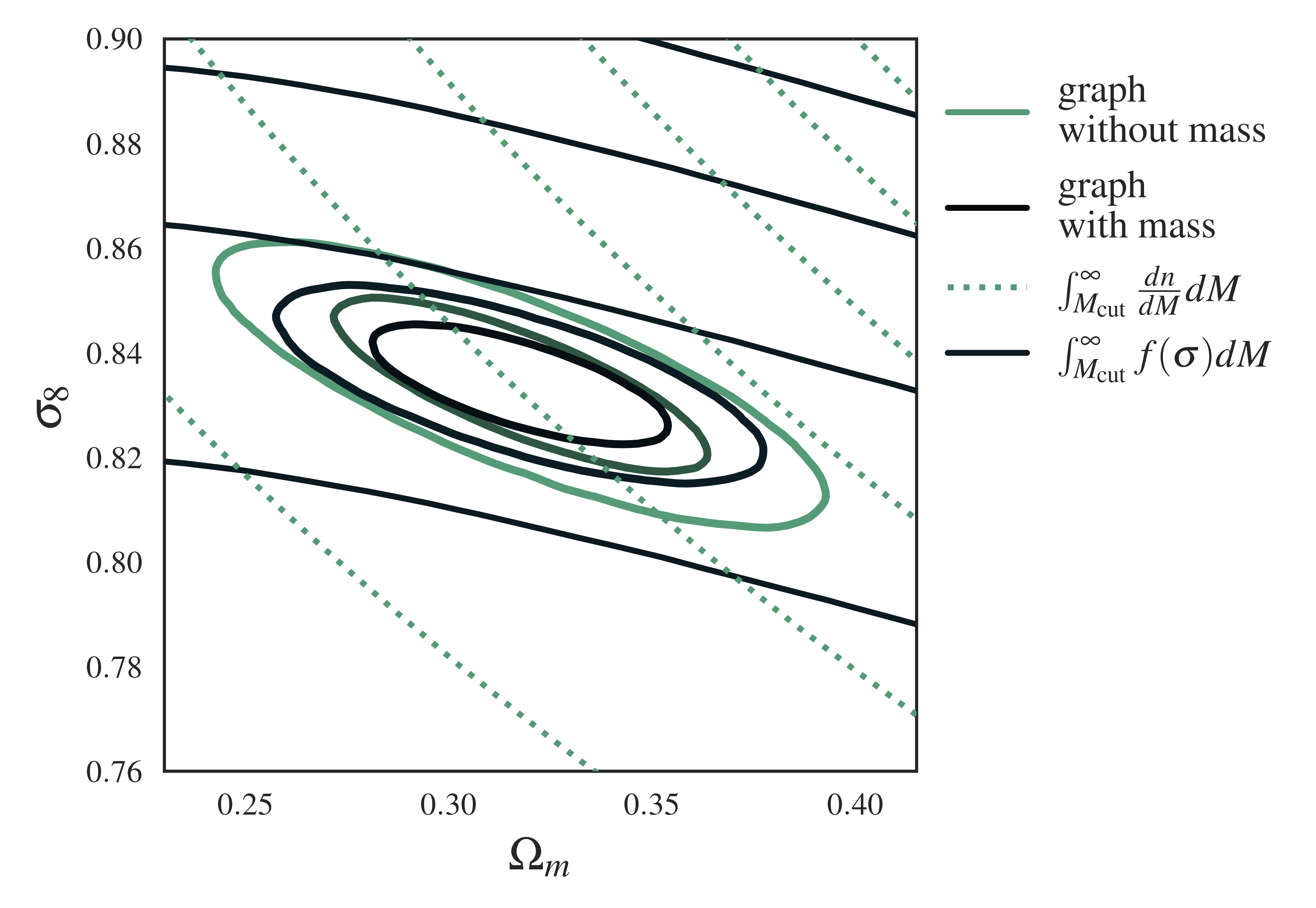
A quick aside: how much information is in a (fixed) statistic ? The plot above is what we call a “Fisher forecast” for cosmological parameters. It shows a Gaussian Approximation to the posterior for a given statistic (or likelihood), which can be plotted as an ellipse. 2PCF is the average clustering information collected by comparing pairs of halos across all the catalogues. We compute the 2PCF Fisher in the same way we compute the gIMNN finite-difference Fisher (except this time with the fixed 2PCF across simulations – no gradient descent here !)

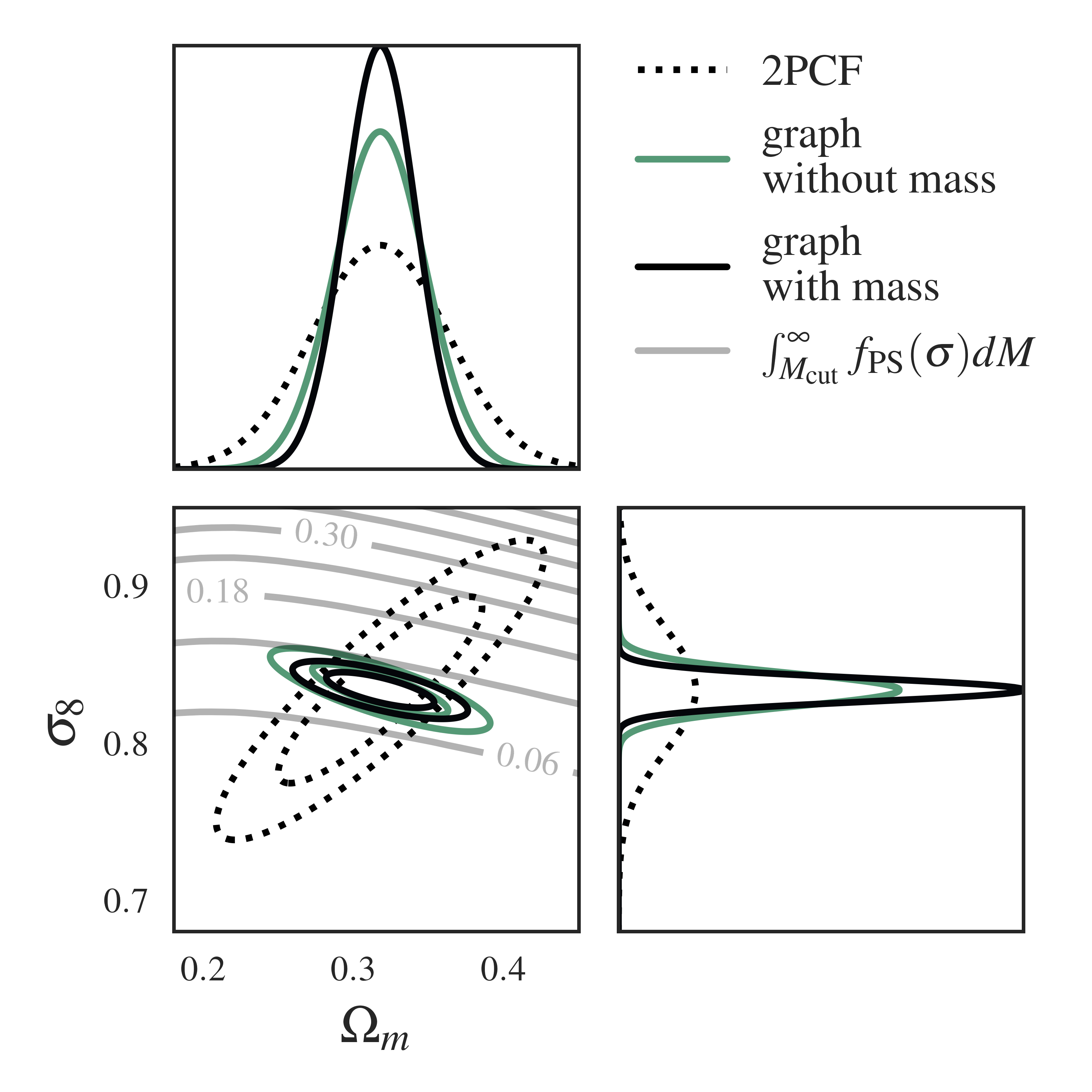
There is a lot going on in this Fisher plot – let’s start with the dotted ellipse. This is the information extracted about the cosmological parameters from just the 2-point correlation function (2PCF), which probes clustering – think of it as our baseline. The grey lines that slice through the 2PCF ellipse are lines of fixed mass computed from a halo mass function, which tells us how the halo mass in the universe changes with changing $(\Omega_m, \sigma_8)$.

Without going into the details, the main takeaway here is that the gIMNNs are able to automatically combine mass and clustering information along the correct axes to better constrain the parameters ! And we’ve done so in an entirely unsupervised manner ! In the paper we show that a lot of this information comes from the changing cardinality or number of halos in the graph.

If you take an even closer look, you’ll see that the Fisher ellipse produced by the annotated graph and gIMNN rotates slightly towards the halo mass function (HMF) lines, away from the halo number density lines, when mass labels are added to the graph nodes.

Halo Mass Function Information

To explain this behaviour, we need to dive into the HMF formalism. The fraction of mass found in halos per unit interval $\ln \sigma^{-1}$ can be parameterized as a function, $f(\sigma)$, called the halo mass function, which obeys

\[\begin{equation} \int_{-\infty}^\infty f(\sigma) d \ln \sigma^{-1} = 1, \end{equation}\]

and can be related to the number density of halos in a given interval, $dn/dM$, via

\[\begin{equation} \frac{dn}{dM} = \frac{\rho_o}{M}\frac{d\ln \sigma^{-1}}{dM} f(\sigma), \end{equation}\]

where $\rho_o$ is the mean mass density of the universe. The form of $f(\sigma; \vartheta)$ can be related analytically to cosmological parameters or approximated using simulations.

If we rearrange the above equation for $f(\sigma)$, we obtain

\[\begin{equation} f(\sigma) = \frac{M}{\rho_o} \frac{dn(M)}{d \ln (\sigma^{-1}(M))}, \end{equation}\]

Integrating the halo number density from a fixed mass $M_{\rm cut}$ yields the number of halos with a mass above this threshold:

\[\begin{equation} N(M_i > M_{\rm cut}) = \int_{M_{\rm cut}}^\infty \frac{dn}{dM} dM, \end{equation}\]

which in our case is the node cardinality of a halo graph, $N^v$. By contrast, integrating the halo mass function from $M_{\rm cut}$ yields the fraction of total mass residing in collapsed halos of mass above $M_{\rm cut}$:

\[\begin{equation} F(M_i > M_{\rm cut}) = \int_{M_{\rm cut}}^\infty f(\sigma) dM, \end{equation}\]

which incorporates both halo number $N^v$ and mass information above $M_{\rm cut}$.

When graphs aren’t decorated with masses, the Fisher ellipse (green) rotates towards the number density contours (dashed lines) $N(M_i > M_{\rm cut})$, since this is the information the network receives: the number of halos above the mass cut.

When we do specify masses, we see the Fisher (black) aligned with the integrated halo mass fraction lines (black lines) – our network has learned this concept automatically !

Part III: A more realistic case: adding survey noise

Now that we know the raw information content of the graph structure, we can see if gIMNNs would be useful for catalogues assembled with noisy halo or galaxy masses. Here we introduce a white noise model to the halo masses before making a catalogue cut at $M_{\rm cut}$: $\begin{equation} \hat{m}_i = m_i + \mathcal{N}(0,\sigma^2_{\rm noise}), \end{equation}$ where $\sigma_{\rm noise}=A_{\rm noise}M_{\rm cut}$ with amplitude $A_{\rm noise}$. Observed halos that fall below $M_{\rm cut}$ are then trimmed from the graph to mimic real catalogue cuts in the presence of noisy mass estimates. We can think of this as a likelihood for a halo finder operating on noisy galaxy mass or luminosity measurements.

We can incorporate this forward model into the gIMNN training scheme such that the network becomes hardened to both the noisy halos and changing catalogue size.

Training Curves

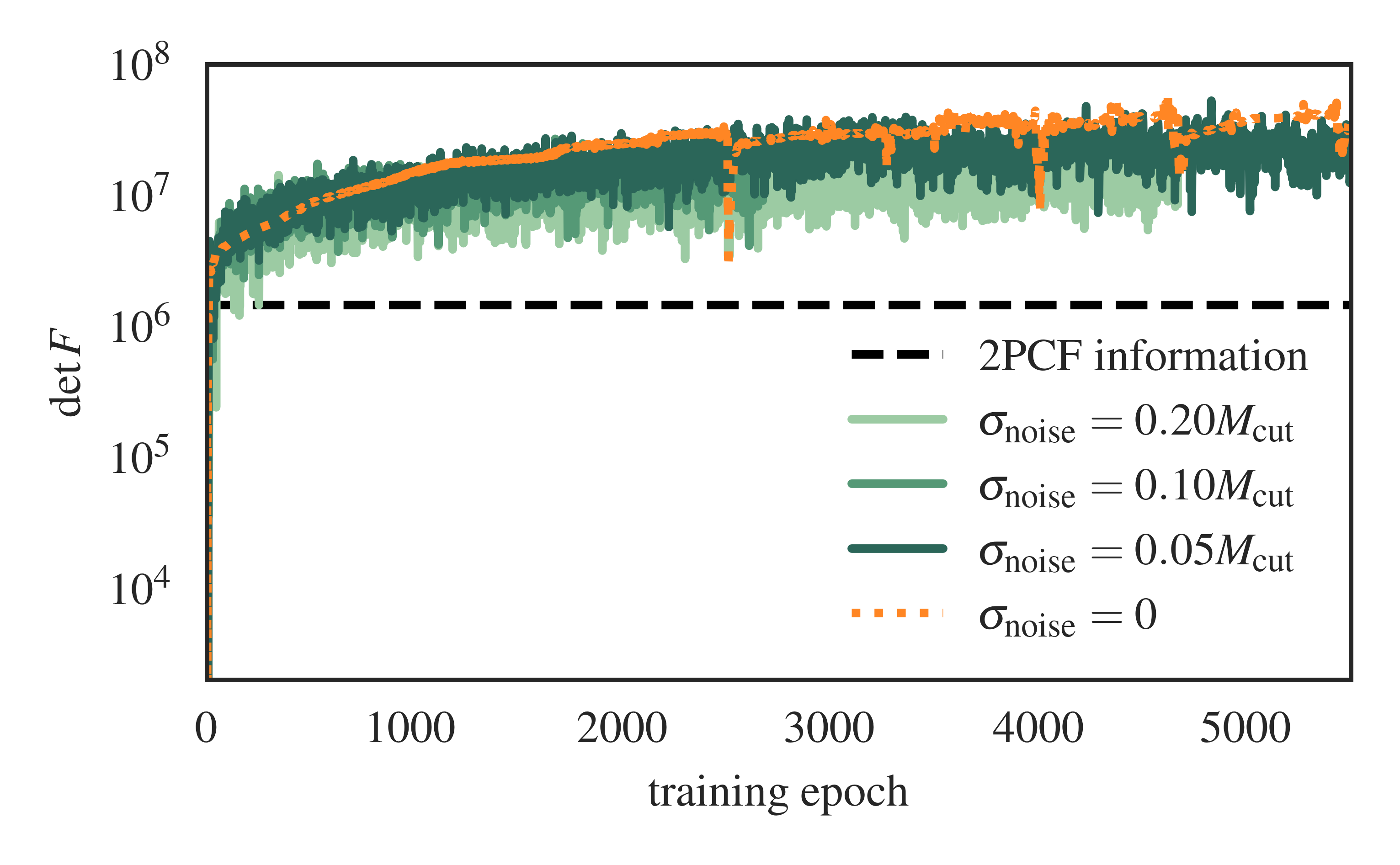
In the above plot we see the effect of increasing the noise amplitude parameter $A_{\rm noise}$ on IMNN training. Intuitively we’d expect the Fisher information estimate to fluctuate more as the lowest-mass halos in the survey become dominated by noise. More noise also means that the catalogue data becomes less informative about the cosmology, so the Fisher information drops slightly for the higher-noise cases. We term this information leakage, resulting in higher uncertainty contours in the Fisher plot:

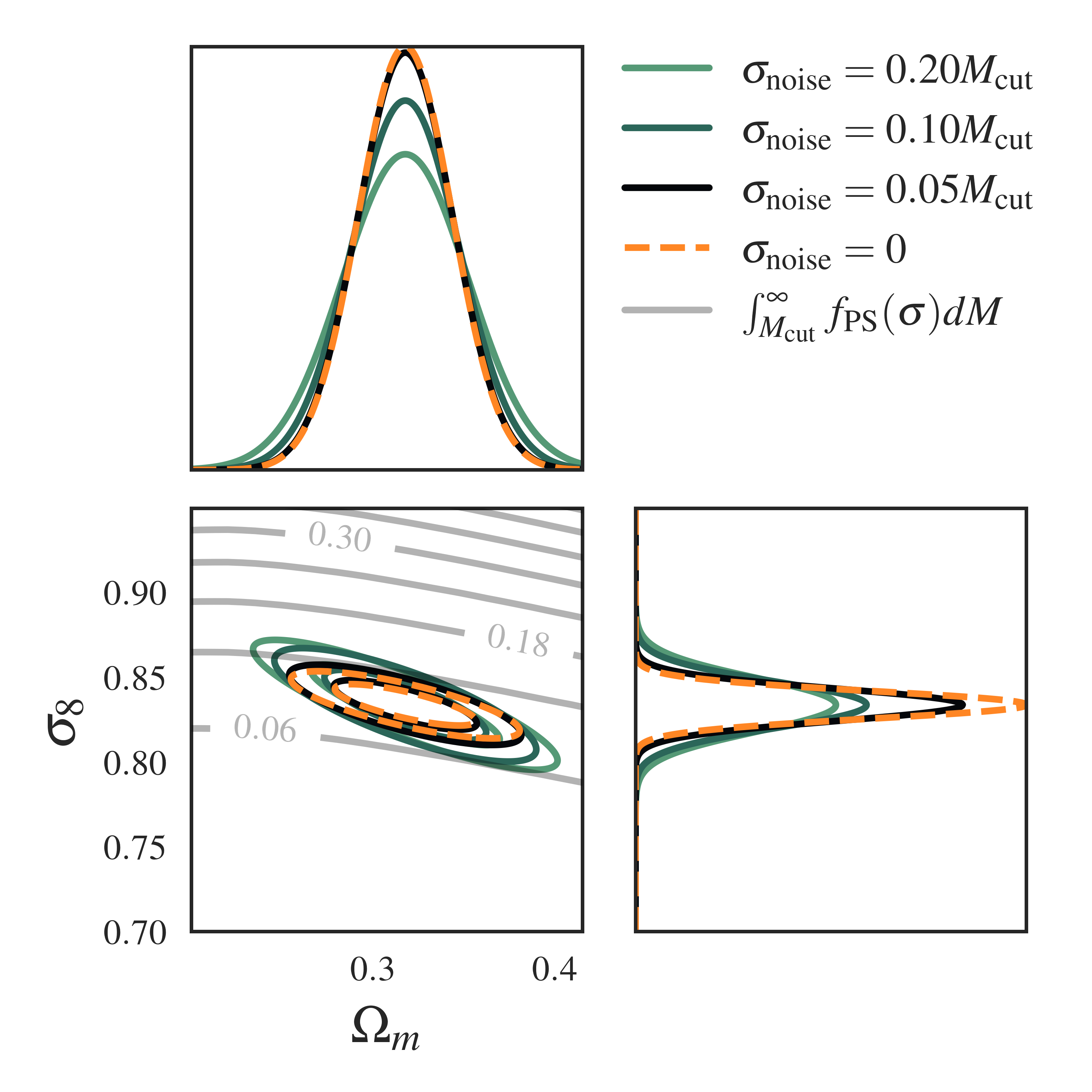
We also plot the HMF lines for comparison and see that as the mass information becomes muddied by noise, the Fisher also tilts away from the HMF line alignment that we observe in the no-noise case (orange).

Simulation-based Inference: How to use gIMNNs in Practice

This is largely an exploratory study to elucidate the information in cosmological catalogues by expressing the data as graphs. Along the way, however, we developed a technology that allows us to compress catalogues into neural summaries, $\textbf{x}$. We can then compare simulated catalogues at different values of $\theta$ to an actual dataset and accept-or-reject the simulations to build a posterior distribution. This scheme is called Approximate Bayesian Computation (ABC), and can be expensive for uninformative summary statistics. An even smarter approach is to use another set of neural networks to parameterize a posterior density. This technique, called Density Estimation Likelihood-Free Inference (DELFI), is what we used for our neural summaries in this paper.

Neural Field-Level Information Extraction. This project is similar in style to field-level Information Maximising Neural Networks. Both works aim to extract cosmological information from LSS. However, in our field-level study we assumed that we had access to the full density field image of a log-normal LSS simulation. We computed the analytic Fisher information for this field and showed that IMNNs with a CNN architecture can saturate the field-level information content–equivalent to writing a likelihood for every single pixel in the image ! We can think of the graph representation as a way to extract cosmological information when we don’t have a complete image of the underlying density field. Alternatively, we can think of images as 2D graphs bound to a lattice !

Closing Thoughts

In this study we investigated how much cosmological information is locked away in dark matter halo catalogues. To do this, we exploited the flexibility and symmetric properties of graphs to efficiently compress massive simulations down to a couple of numbers using graph neural networks.

The language of graphs is an elegant way to describe the unintuitive nature of large-scale structure. Equipped with the technology of graph neural networks and a rigorous stastical metric (the Fisher information), we were able to cast cosmology as an optimization problem and find a way to squeeze more information out of catalogues than traditional statistics. We worked with really small catalogues, but demonstrated that even these structures are very sensitive to cosmology.

We introduced new vocabulary with which to describe the cosmic web, and incorporated graph learning in the context of cosmological statistics. The extensions to this work are numerous, both within and outside of cosmology.